TL;DR: Calibration Boosts Accuracy
We tested our new calibration ensemble across ~18,000 predictions from our 30m+ parameter model. Here's what matters for traders relying on MarketCrunch AI for their daily trading signals:
- 📉 76.8% reduction in average prediction error- sharper, more dependable signals.
- 🎯 Errors now cluster near zero, cutting down costly outliers.
- 📊 Better accuracy on 4 of 5 trading days,
Bottom line: You get clearer, more reliable signals to trade with confidence in any market condition.
— - - - - - - - - - - - - - - - - - - - - - - - - - - - - - - - - - - - - -
Ensemble Calibration Methods
In Measuring Market's Mood with Dynamic Volatility: An Apple Inc. Case Study , we explored the crucial first step in our calibration process: measuring the market's "mood" by forecasting volatility. We saw how the GARCH family of models [1] gives us a dynamic, forward-looking view of risk, which is far superior to relying on simple historical averages.
But a raw forecast, even a volatility-aware one, is like a powerful engine without a steering wheel. It has potential, but it's not yet ready for the road. Models, like people, can have inherent biases or fail to adapt to rapidly changing conditions. The final, critical step is calibration: the process of intelligently adjusting a raw forecast to correct for its flaws and align it with reality.
This isn't about simply nudging a number up or down. It's a sophisticated, multi-pronged strategy. We run three distinct calibration methods in parallel, each designed to tackle the problem from a different angle. Let's break them down.
Method 1: The Adaptable Strategist - A Two-Regime Approach
Markets don't have a single personality. They switch between periods of calm and periods of chaos. Our first calibration method recognizes this and adapts its strategy accordingly. It uses our GARCH volatility forecast to determine if we are in a "high volatility" or "normal volatility" regime and applies a different technique for each.
In High Volatility Regimes: We Harness the Storm
When the market is turbulent, price movements are often larger and more exaggerated. To keep pace, our model becomes more aggressive. This method takes our GARCH volatility forecast and uses it to scale the predicted price change. If volatility is high, it amplifies the model's raw prediction, allowing it to capture the bigger swings that are common during market storms. It's like a sailor adjusting the sails - more wind (volatility) requires a different trim to effectively harness that power.
In Normal Volatility Regimes: We Correct the Aim
Even in calm markets, a model can have systematic biases - a tendency to consistently overestimate small gains or underestimate small losses, for example. To correct this, we use a statistical technique called Isotonic Regression [2].
Think of it like a bathroom scale that's slightly off. Every time you step on it, it adds an extra two pounds or subtracts one. You can still see if you're generally gaining or losing weight, but the absolute number is biased. Isotonic regression is the calibration step where we check the scale against known weights and adjust it.
The key feature of this technique is that it's monotonic. This means it preserves the relative ordering of predictions: if the raw model says one outcome should be higher than another, the calibrated predictions will keep that order. What changes is the magnitude of the forecast. A predicted +2% move might be adjusted to +1.2%, but it will still sit above a predicted +1% move (which might be calibrated to +0.8%). In other words, isotonic regression corrects the bias in the size of the move without scrambling the model's sense of direction.
Method 2: A Smooth Blend - Hybrid approach
Our second method takes a different philosophical approach. Instead of a hard switch between two states, it creates a smooth blend of bias correction and volatility adjustment.
It works in two steps:
- Always Correct for Bias: First, it applies the same Isotonic Regression we saw before. The logic here is that a model's systematic biases should always be corrected, regardless of the market's mood.
- Apply a Weighted Volatility Adjustment: This is the clever part. Rather than a simple on/off switch, this method calculates a volatility weight using a Sigmoid function [3].
A sigmoid function produces a smooth S-shaped curve that goes from 0 to 1. When our GARCH forecast shows low volatility, the sigmoid weight is near 0, and the volatility adjustment has almost no effect. As volatility increases, the weight smoothly climbs towards 1, applying the volatility adjustment with progressively more intensity.
This hybrid approach is less like a light switch and more like a gas pedal. It applies the power of the volatility adjustment smoothly and proportionally, resulting in a more nuanced and stable calibration.
Method 3: The Advanced Method - A Machine Learning-Powered Calibration
Our third and most sophisticated method treats calibration itself as a machine learning problem. Instead of using a simple rule, it deploys a dedicated regression model to learn the complex patterns of our main model's errors.
The key difference is the richness of the data it uses. This calibration model considers not just the raw prediction, but a whole host of features, including:
- The GARCH volatility forecast.
- Rolling statistics of past errors: What was the main model's average error over the last 10 days? How much did that error vary? This helps the calibration model understand if the main model is currently performing well or has recently been drifting off course.
It then feeds these features into a well-known statistical model such as XGBoost [4] or a Quantile Regression [5] model. While standard regression predicts the single most likely outcome, this approach can predict a range of possibilities. For instance, it can simultaneously predict the 10th, 50th (median), and 90th percentile outcomes. This gives us a much richer understanding of the prediction's potential uncertainty, not just a single point estimate.
This is like a master diagnostician who, instead of looking at one symptom, reviews the patient's entire chart - recent history, vital signs, and more - to make a much more informed and reliable diagnosis.
Putting It All Together
We don't bet on a single horse. We run all three of these calibration methods in parallel for every single prediction. But what do we do with three different results? We combine them.
We create a final prediction using a weighted average of their outputs. Based on extensive backtesting, we assign a higher weight to the models that have historically proven most reliable.
This technique, known as ensembling, makes our final prediction more robust. By combining the "opinions" of different specialist models, we reduce the risk of being misled by any single model's quirks.
This layered, multi-faceted calibration process is how we turn a raw forecast into a reliable, self-aware, and actionable insight, ready to navigate the complexities of the real-world market.
Results in Action: How Our Strategy Performs
Talk is cheap, so let's look at the real-world results of our new calibration ensemble. We A/B test our new models ("Treatment") against our previous best ("Control"). The results speak for themselves.
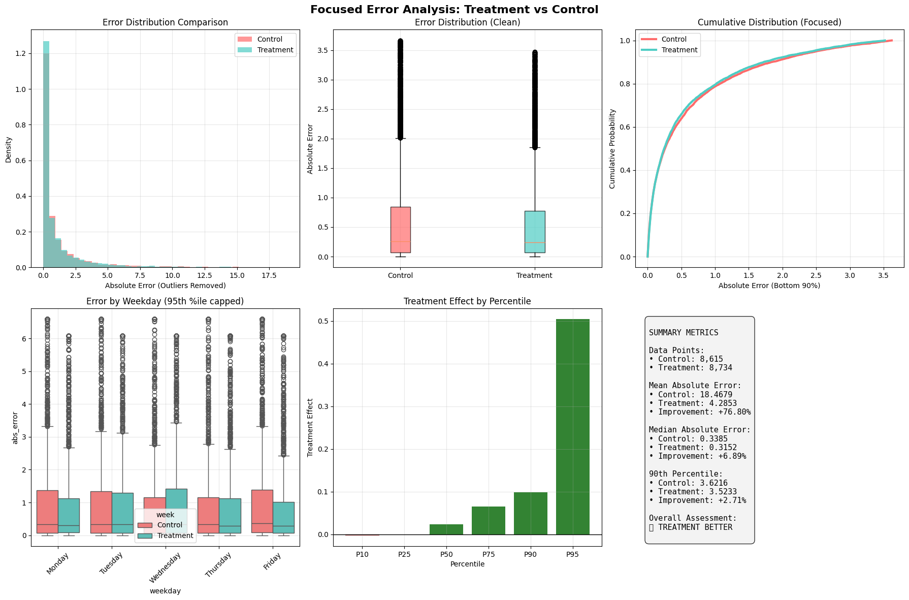
The charts above show a head-to-head comparison over nearly 18,000 predictions.
- Summary Metrics show a staggering 76.8% improvement in Mean Absolute Error (MAE). This massive improvement is driven by the model's ability to tame extreme outliers, which is confirmed in the "Treatment Effect by Percentile" chart - the error reduction is largest for the most inaccurate predictions.
- The Error Distribution (top left) shows our new model's errors (teal) are sharply concentrated near zero, while the old model (red) had a "fatter tail" of large, costly errors.
- The Cumulative Distribution (top right) is even clearer. The teal line's position shows that for any given error level, a higher percentage of our new model's predictions fall below it.
A look at a recent week shows this consistency. Our new calibration strategy led to a lower Mean Absolute Error on 4 out of 5 days, with dramatic improvements on Monday (25.39 MAE reduction), Thursday (21.64), and Friday (22.48).
The Road Ahead: Evolving Our Calibration Strategy
Like markets, models evolve. We're working on dynamic weighting systems that learn in real-time, which calibration expert to trust most. And we're expanding our toolkit with sentiment, options data, and sequence-aware models (LSTMs, Transformers).
Who are we?
MarketCrunch AI is built by a mission-driven team of engineers, quants, and researchers from MAANG, high-frequency trading, and applied ML labs. We've shipped real-time systems, tuned signals in microseconds, and built AI that scales under pressure.
Our goal? Level the playing field by turning raw market data into fast, explainable, and actionable insights for every investor.
References
[1] Bauwens, Luc, Sébastien Laurent, and Jeroen VK Rombouts. "Multivariate GARCH models: a survey." Journal of applied econometrics 21, no. 1 (2006): 79–109.
[2] Barlow, Richard E., and Hugh D. Brunk. "The isotonic regression problem and its dual." Journal of the American Statistical Association 67, no. 337 (1972): 140–147.
[3] Kyurkchiev, Nikolay, and Svetoslav Markov. "Sigmoid functions: some approximation and modelling aspects." LAP LAMBERT Academic Publishing, Saarbrucken 4 (2015): 34.
[4] Chen, Tianqi, and Carlos Guestrin. "Xgboost: A scalable tree boosting system." In Proceedings of the 22nd acm sigkdd international conference on knowledge discovery and data mining, pp. 785–794. 2016.
[5] Koenker, Roger, and Kevin F. Hallock. "Quantile regression." Journal of economic perspectives 15, no. 4 (2001): 143–156.
[6] Graves, Alex. "Long short-term memory." Supervised sequence labelling with recurrent neural networks (2012): 37–45.
[7] Wen, Qingsong, Tian Zhou, Chaoli Zhang, Weiqi Chen, Ziqing Ma, Junchi Yan, and Liang Sun. "Transformers in time series: A survey." arXiv preprint arXiv:2202.07125 (2022).