How MarketCrunch AI uses Black-Scholes, volatility surface modeling, and exhaustive grid search to transform stock predictions into optimal options plays
A Quick Summary: Navigating Strike, Time, and Direction
How MarketCrunch AI comes up with Options Trade Ideas ? Turning a stock forecast into an options trade is a search problem across strike, expiry, and call/put-where intuition breaks fast. In this post, I'll show the engine we built to solve that systematically: We price every liquid contract under one consistent model, compare today's theoretical price to the price under a predicted next-close, and rank contracts by expected return. We also apply a simple term-structure volatility adjustment for short-dated options and filter for tradability.
What you'll see A real GOOGL example that connects the engine's estimate to a trade we actually executed. Then I'll explain why we exited around ~16% instead of chasing the theoretical max.
What you'll learn MAI provides a strong edge in identifying the setup and ranking contracts. From there, traders can tailor outcomes with their own rules, such as position sizing, execution discipline, and exits, especially when real markets diverge from the model (IV crush, wide spreads, or gap moves).
The Theoretical Foundation: Black-Scholes-Merton Model
At the heart of our engine sits the Black-Scholes-Merton equation, the 1973 breakthrough that won Myron Scholes and Robert Merton the Nobel Prize (Black had passed away). The beauty of Black-Scholes is that it reduces option pricing to five observable inputs:
Call Option Pricing
The theoretical price of a European call option is:
Put Option Pricing
The formula inverts:
What This Actually Means
The formula is elegant in its logic:
The natural log term ln( S / K ) is doing something subtle: it measures the moneyness of the option on a logarithmic scale. An option that's 10% out-of-the-money ( K=1.1S ) has the same mathematical character as one that's 10% in-the-money ( K=0.9S ), just inverted.
The formula outputs a theoretical "fair price" for the option right now. But here's what makes it powerful for our use case: we can run it twice.
The Two-Price Trick
For every option contract, we calculate:
- Price today using the current stock price S and time T
- Price tomorrow using predicted stock price S' and time T - 1/365
The difference between these prices, divided by today's price, gives us the expected percentage gain.
This is conceptually simple but computationally intensive. Running Black-Scholes 643 times for a single stock prediction, twice per option (before/after), means executing the formula 1,286 times. And it needs to complete fast enough to maintain a responsive user experience.
The Volatility Problem: Why Historical Vol Isn't Enough
Here's where traditional options calculators fall short. They use a single volatility number for all expirations. But in reality, short-dated options exhibit significantly higher implied volatility than long-dated ones.
This phenomenon, called the volatility term structure, has deep roots in market microstructure:
Why Short-Term Options Are More Volatile
- Event Risk Concentration: A near-term option is exposed to just one or two significant events. Miss one earnings report, and you're done. Longer options can weather multiple events.
- Gamma Risk: Market makers charge a premium for the convexity of short-dated options. When expiration is days away, delta can swing wildly with small price moves.
- Information Asymmetry: Short-term option buyers often know something. This adverse selection gets priced in.
Our Volatility Model: Exponential Decay
We model this with an exponential multiplier that decays with time:
Where T is days to expiration and σ_base is 30-day historical volatility.
This gives us:
- 1-day expiry: ~3.0x base volatility
- 7-day expiry: ~1.7x base volatility
- 30-day expiry: ~1.1x base volatility
- 90+ day expiry: ~1.0x base volatility (no adjustment)
The decay constant of 7 days was calibrated empirically by analyzing thousands of options trades. It represents the half-life of the term structure premium.
Computing Base Volatility
For the base volatility, we calculate 30-day historical volatility using the standard formula:
Why log returns instead of arithmetic? Because they're time-additive and symmetric. A 10% gain followed by a 10% loss doesn't net to zero-you end up down. Log returns fix this.
The 252^.5 factor annualizes the daily volatility (252 trading days per year). This matches how options are priced in the market.
The Engineering Challenges: Making It Fast
Calculating 1,600 Black-Scholes prices in seconds requires careful engineering.
Challenge 1: Computational Efficiency
Black-Scholes involves expensive operations: natural logs, exponentials, and cumulative normal distribution lookups. We optimized:
- Pre-computed volatility multipliers: Saved 40%
- Early termination: If T ≤0 (expired option), return intrinsic value immediately. Skip all calculations.
Challenge 2: Database Performance
Fetching 30 days of historical prices for volatility calculation hits PostgreSQL. We optimized:
- Connection pooling: Reuse connections instead of creating new ones per request
- Denormalized storage: Store close prices in a dedicated table, pre-sorted by date
Challenge 3: API Latency
Our broker's options contracts API can be slow (300ms+ for 800 contracts). We mitigate:
- Caching: Contract metadata is cached for 10 minutes; pricing inputs refresh more often because options quotes can change quickly.
- Parallel requests: When fetching current price + options + historical data, we fire all requests in parallel
- Fallback endpoints: Try multiple API endpoints in sequence if one fails
Challenge 4: Numerical Stability
Black-Scholes breaks down in edge cases:
- T≈0: Division by T explodes. Solution: Return intrinsic value when T<0.001
- σ→0: Formula is undefined at zero volatility. Solution: Floor volatility at 10%
- S/K≫1or≪1: Deep ITM/OTM options have d1values beyond ±10. Solution: Clamp d1to [-10, 10] to prevent overflow
The PnL Surface Visualization: Extending to 2D
Then we take it even further. Instead of calculating gain at one predicted price, we calculate gain across a grid of possible prices.
We build a price grid spanning ±20% of the current price:
- Range: [S⋅0.8,S⋅1.2]
- Steps: 60 points
- Step size: (S⋅1.2−S⋅0.8)/59
For each option and each grid point, we calculate P&L:
PnL(S_grid) = [max(0, S_grid - K) - premium_paid] · 100 shares
This produces a surface plot showing how profit evolves across :
- X-axis: Underlying stock price
- Y-axis: Profit/loss
- Z-axis: Various strikes & expiry
Users can visualize the entire risk profile at a glance.
Why This Matters
The surface reveals non-obvious insights:
- Maximum profit zones: Where the option makes the most money
- Break-even points: Exactly where the stock needs to move to avoid loss
- Loss limits: For spreads, where losses cap out
It's like seeing the entire probability distribution of outcomes, not just the single predicted path.
Real trade: from an estimate on MarketCrunch AI → Robinhood
The screenshot at the top of this post wasn't a mock. We implemented the setup that turns an overnight stock pick into a specific options candidate. Then I executed the trade and recorded the receipts.
Selection (overnight): Our AI models flagged GOOGL as a pick for Feb 9.
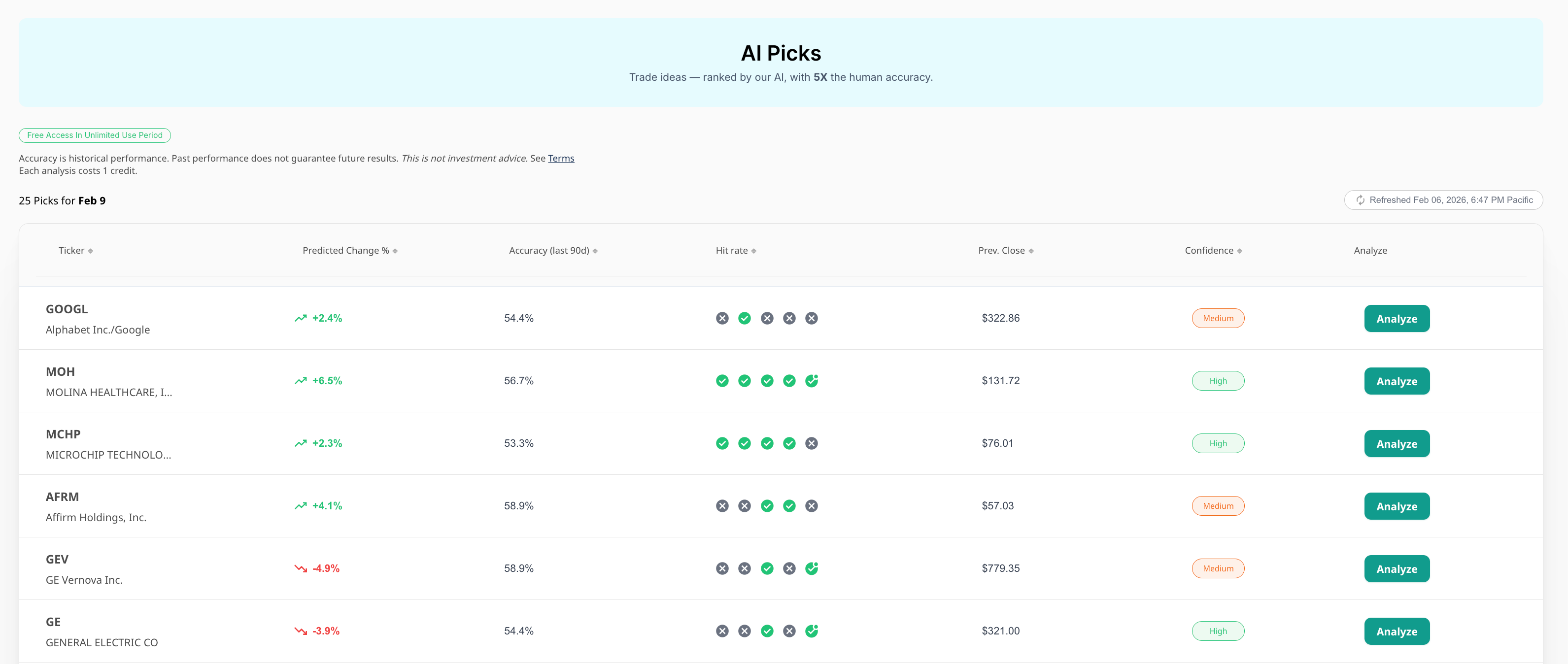
Research (in-app): After clicking Analyze, the engine surfaced this setup:
- Contract: GOOGL $342.50 Call, Exp 2/20, 11 DTE
- At a target price of $330.64, the tool estimated 100%+ upside (profit probability shown: 31%).
Execution: Receipts :
- Buy: 2 contracts filled at $1.51 (total cost $302.08) on 2/9 6:30 AM PST
- Sell: 2 contracts filled at $1.75 (credit $349.92) on 2/9 8:16 AM PST
- Realized profit: +$48, which is about +15.9% on capital used (48 / 302.08).
Why we exited early (risk management > chasing the max)
Our engine ranks contracts under a modeled move, and sometimes that model may imply"100%+" upside. But the trader's job is deciding what's worth holding. We exited around ~16% because options are path-dependent, time decay is relentless, and the last stretch of "theoretical upside" usually carries the most risk.
We provide the setup by ranking contracts objectively. Traders personalize the outcome through risk management: sizing and exits.
Limitations & failure modes (read this before you copy a trade)
This engine ranks options under assumptions. If those assumptions break, the "best" contract can flip.
Model limitations
- European model approximation: Black-Scholes is European; many single-stock options are American-style, so early exercise/assignment effects (esp. dividends, deep ITM, near expiry) aren't fully captured.
- No jump/gap modeling: Overnight gaps and event jumps violate diffusion assumptions.
Volatility limitations
- We don't predict IV changes; we assume volatility stays constant before and after the move (conservative, but imperfect).
- Term structure isn't a full surface: skew/smile by strike can matter a lot.
Execution limitations
- Spreads and slippage: the theoretical edge can vanish if the bid-ask is wide or fills are poor.
- Liquidity: low-volume strikes can "win" on paper but be untradeable (we filter illiquid contracts).
Future Enhancements: The Research Roadmap
A few upgrades are already on the roadmap:
- Better vol forecasting (moving beyond historical vol)
- Multi-leg optimization (spreads/condors/calendars)
- Liquidity-aware ranking (bid-ask, volume, OI thresholds)
The Bottom Line: Math Over Intuition
Options are mathematical instruments. If you have a stock forecast, the most reliable way to translate it into an options play is to compute the outcomes exhaustively, account for basic market realities like time decay and term structure, and rank contracts objectively - instead of guessing. Then the trader layers on the personal edge: sizing, execution, and exits to match their own risk tolerance.
Questions about our implementation? We're always happy to discuss the technical details. This is where finance meets computer science, and we love both.Email us: trading@marketcrunch.ai
References
Foundations
- Black, F. & Scholes, M. (1973). The Pricing of Options and Corporate Liabilities.
- Merton, R. C. (1973). Theory of Rational Option Pricing.
- Nobel Prize in Economic Sciences (1997). Press release on option pricing.
Volatility surface & modern modeling 4. Gatheral, J. The Volatility Surface: A Practitioner's Guide. 5. Heston, S. (1993). A Closed-Form Solution for Options with Stochastic Volatility. 6. Dupire, B. (1994). Pricing with a Smile. 7. Hagan et al. (2002). Managing Smile Risk (SABR). 8. Bergomi, L. Stochastic Volatility Modeling. 9. Gatheral, J., Jaisson, T., Rosenbaum, M. (2014). Volatility Is Rough.
Systematic options & risk 10. Natenberg, S. Option Volatility & Pricing. 11. Sinclair, E. Volatility Trading. 12. Hull, J. Options, Futures, and Other Derivatives.
Market structure & guardrails 13. Harris, L. Trading and Exchanges. 14. Options Clearing Corporation. Characteristics and Risks of Standardized Options (ODD). 15. Cboe Global Markets. VIX Methodology.
About us
- MarketCrunch AI on Pitchbook and Crunchbase
- Producthunt launch
- Follows on LinkedIn and X (formerly Twitter)